Time series data is structured data where the index column is date-time data (a Series or DataFrame). This section introduces the organization of time series data.
Overview of Time Series Data
Many people confuse time series data with date-time data — they are actually completely different types. Date-time data is a basic data type, while time series data is structured data (a Series or DataFrame with a date-time index column).
In the pandas package, you can use the date_range function to generate time series data using a given start time, interval unit, and number of data points.
In the worksheet shown in Figure 5-49, enter the following code in Python mode in the formula bar of cell A1:
start_time = pd.to_datetime('2022-03-18 00:00:00')
data = np.random.randint(1, 11, size=100)
time_series = pd.date_range(start=start_time, periods=100, freq='H', name='Time')
series_data = pd.Series(data, index=time_series, name='Measurement Value')
Press Ctrl+Enter. Cell A1 returns a Series object. Displaying it as Excel values (columns A-B in Figure 5-49) — the code generates 100 date-time data points starting from the given time with an hourly interval, uses NumPy’s random.randint to generate 100 random integers between 1–10 as measurement values, and combines them into a Series (time series data).
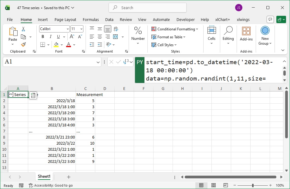
Figure 5-49 Generating Time Series Data
Data Filtering
Time series data is essentially a Series or DataFrame with a date-time index, so all attributes and methods of Series/DataFrame objects apply to time series data.
In the worksheet shown in Figure 5-50, columns A-B show daily product sales over a period. We need to filter dates with sales ≥ 20. Enter the following code in Python mode in the formula bar of cell D1:
df = xl("A1:B31", headers=True)
df[df['Sales'] >= 20]
Press Ctrl+Enter. Cell D1 returns a DataFrame object. Displaying the content (columns E-G in Figure 5-50) shows the sales dates with values ≥ 20.
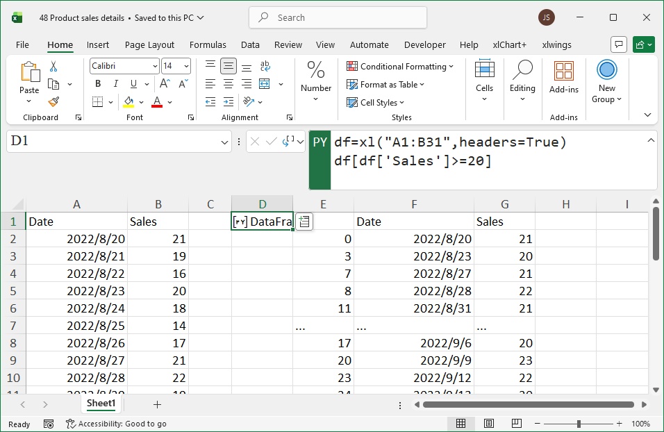
Figure 5-50 Filtering Data
Data Shifting
Given a date-time sequence and a date-time interval, you can quickly obtain a shifted date-time sequence. The interval can be a regular date or a business day.
In the worksheet shown in Figure 5-51, columns A-C show employees’ vacation schedules (start date and duration). We need to calculate the end date. Enter the following code in Python mode in the formula bar of cell D1:
df = xl("A1:C7", headers=True)
df['Vacation End Date'] = df.apply(lambda x: x.Vacation Start Date + pd.DateOffset(days=x.Vacation Duration), axis=1)
df
Press Ctrl+Enter. Cell D1 returns a DataFrame object. Displaying the content (columns E-H in Figure 5-51) shows the calculated end dates. The code uses an anonymous function and DataFrame.apply to shift the start date by the vacation duration (via pd.DateOffset).
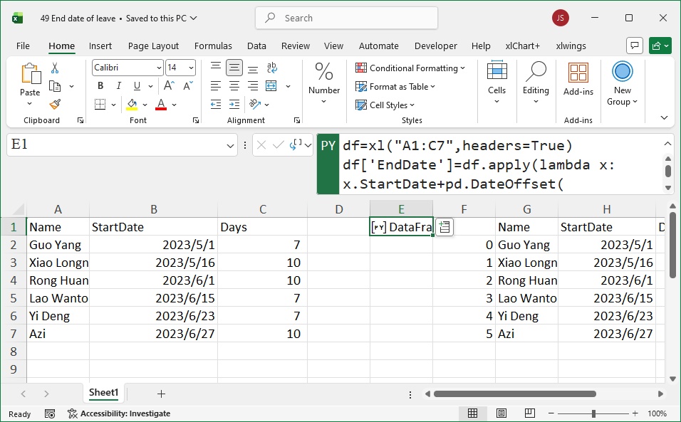
Figure 5-51 Calculating Vacation End Date
Data Resampling
For a given time series, you can resample it at a specified frequency and aggregate using a specified function. In the worksheet shown in Figure 5-52, columns A-B show hourly measurements. We need to resample to daily data (daily value = mean of hourly values that day). Enter the following code in Python mode in the formula bar of cell D1:
df = xl("A1:B101", headers=True)Set the "Time" column as the index
df = df.set_index('Time')Resample by day, use mean for aggregation, round to 2 decimal places
df2 = df.resample('D').mean().round(2)Press Ctrl+Enter. Cell D1 returns a DataFrame object. Displaying the content (columns E-F in Figure 5-52) shows the daily means. The code uses set_index to set "Time" as the index, then resample('D') to group by day and mean() to compute the average.
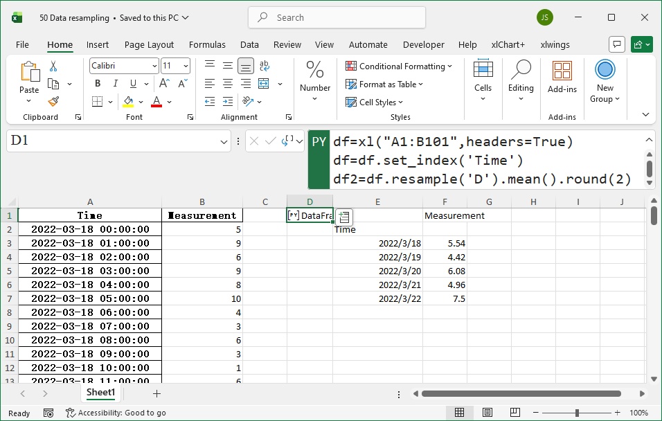
Figure 5-52 Data Resampling
Data Smoothing
Time series data can be smoothed using a moving average window. The method involves defining a sliding window of a specified size. For example, if the window size is 5, it covers 5 consecutive data points in the time series. The center value of the window is taken as the average of all values within the window. Sometimes the median of the window is used instead.
In the worksheet shown in Figure 5-53, columns A-B contain hourly measurements. We need to smooth the data with a window size of 5. Enter the following code in Python mode in the formula bar of cell C1:
df = xl("A1:B101", headers=True)
# Set the "Time" column as the index
df = df.set_index('Time')
# Calculate the moving average with window size 5
smoothed_data = df.rolling(window=5).mean()
# Plot raw data as a green solid line
plt.plot(df.index, df.values, 'g-', label='Raw Data')
# Plot smoothed data as a red solid line with star markers
plt.plot(smoothed_data.index, smoothed_data.values, 'r-*', label='Smoothed Data', linewidth=2)
# Set font sizes for labels and legend to 16 points
plt.xlabel('Time', fontsize=16)
plt.xticks(fontsize=16)
plt.yticks(fontsize=16)
plt.legend(fontsize=16)
Press Ctrl+Enter. Cell C1 returns an Image object. Display it in the merged cell range D1:I19 (as shown in Figure 5-53). The code sets “Time” as the index, applies a rolling window of size 5 for smoothing, and plots both raw and smoothed data. The smoothed line has smaller fluctuations and appears much smoother.
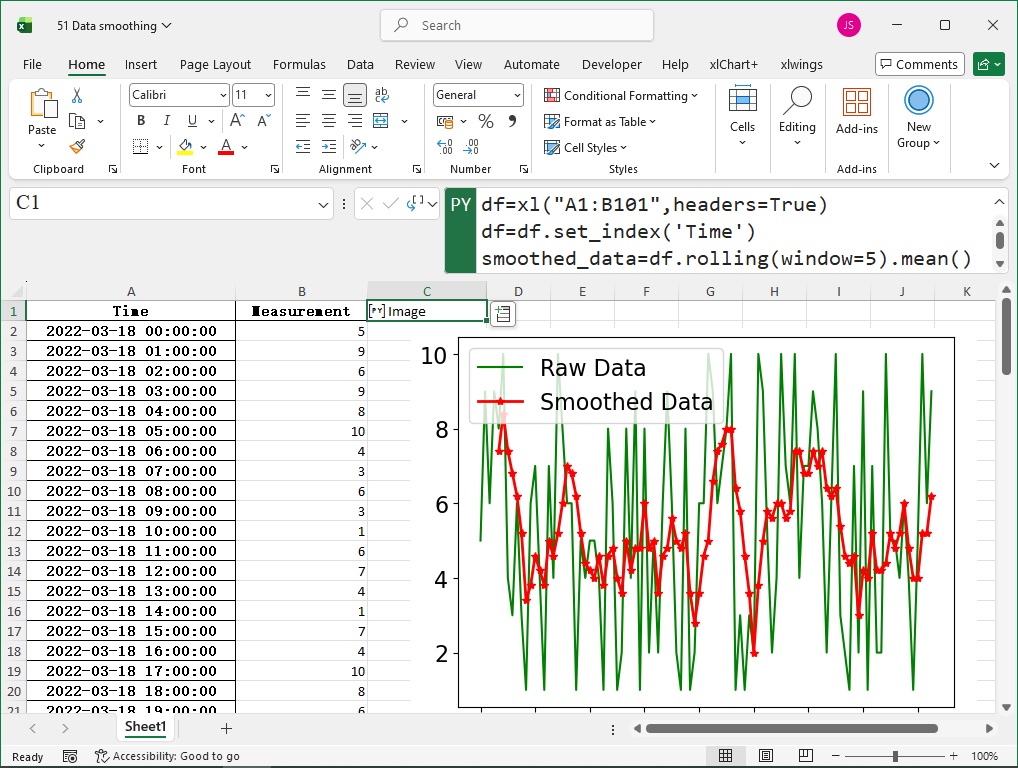
Figure 5-53 Data Smoothing