Data Preprocessing

Handling Duplicate Data

Before statistical analysis, if duplicate data is found and should not exist, it must be handled first. The usual approach is direct deletion. There are two ways to judge row duplication:

A row is considered duplicate if all its values match another row.

A row is considered duplicate if specified columns match those of another row.

In the worksheet shown in Figure 5-54, columns A-C contain some employees’ ID numbers. We need to delete completely duplicate rows. Enter the following code in Python mode in the formula bar of cell D1:

df = xl("A1:C13", headers=True)
df2 = df.drop_duplicates()

Press Ctrl+Enter. Cell D1 returns a DataFrame object. As shown in columns E-G of Figure 5-54, two fully duplicate rows are removed. The drop_duplicates() method deletes duplicate rows.

To judge duplicates based on the “Employee ID” column (rows with the same Employee ID are considered duplicates), enter the following code in Python mode in cell I1:

df3 = df.drop_duplicates(subset=['Employee ID'], keep='first')

Press Ctrl+Enter. Cell I1 returns a DataFrame object. As shown in columns J-L of Figure 5-54, only unique Employee IDs remain. Here, subset=['Employee ID'] specifies using the Employee ID as the criterion, and keep='first' retains the first occurrence of duplicates.

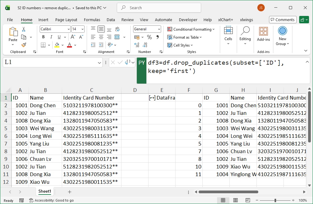
Figure 5-54 Handling Duplicate Data

Handling Missing Values

During data collection, missing values occur when data cannot be collected due to limitations or is lost afterward. Missing values are not zeros — they are empty positions. They prevent proper data processing, so they must be handled by either deletion or filling with specified values.

In the worksheet shown in Figure 5-55, columns A-B contain students’ Chinese exam scores, with some missing due to absence. We need to find the IDs of absent students. Enter the following code in Python mode in cell C1:

df = xl("A1:B21", headers=True)
# Identify rows with any missing values
is_missing = df.isna().any(axis=1)
# Extract IDs of rows with missing values
missing = df[is_missing]['Student ID']

Press Ctrl+Enter. Cell C1 returns a Series object. As shown in column D of Figure 5-55, four students were absent. The code uses isna() to locate missing entries, then indexes the DataFrame to get their Student IDs.

To delete rows of absent students, enter the following code in cell F1:

df2 = df.dropna()

Press Ctrl+Enter. Cell F1 returns a DataFrame object (columns F-G in Figure 5-55), with rows containing missing values removed.

However, simply deleting rows may lose useful information. Therefore, consider filling missing values with nearby values, column mean/median, or fixed values. Enter the following code in cell I1:

df3 = df.fillna(method='ffill')

Press Ctrl+Enter. Cell I1 returns a DataFrame object (columns I-J in Figure 5-55), where missing values are filled with the preceding value (method='ffill').

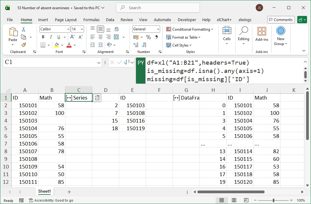
Figure 5-55 Handling Missing Values

Handling Outliers

Outliers are values that are statistically too large or too small due to certain reasons. Including them in analysis can affect results.

There are several methods to detect outliers. Three common ones are introduced below:

Quantile method: Compute the interquartile range (IQR = Q3 − Q1). Values outside [Q1 − 1.5×IQR, Q3 + 1.5×IQR] are outliers.

Mean and standard deviation method: Values outside [mean − 3×std, mean + 3×std] are outliers.

Box plot method: Visually identify outliers beyond the whiskers.

First, using the quantile method. In the worksheet shown in Figure 5-56, column A contains measurement values. Find outliers. Enter the following code in cell C1:

df = xl("A1:A25", headers=True)
Q1 = df['x'].quantile(0.25)    # 25th percentile
Q3 = df['x'].quantile(0.75)    # 75th percentile
IQR = Q3 - Q1                   # Interquartile range
lower = Q1 - 1.5 * IQR          # Lower bound
upper = Q3 + 1.5 * IQR          # Upper bound
outliers = df[(df['x'] < lower) | (df[&#x27;x'] > upper)]  # Boolean indexing

Press Ctrl+Enter. Cell C1 returns a DataFrame (cells D2:D3 in Figure 5-56), showing two outliers: 3 and 326.

Using mean and standard deviation (cell F1):

df = xl("A1:A25", headers=True)
mean = df['x'].mean()
std_dev = df['x'].std()
th = 3 * std_dev
outliers = df[(df['x'] - mean).abs() > th]

This finds one outlier: 326.

Third method: box plot (cell C5):

plt.boxplot(df['x'], vert=True)
plt.xticks(fontsize=16)
plt.yticks(fontsize=16)

Cell C5 returns an Image object (merged region D5:H16 in Figure 5-56), showing two outliers via the box plot.

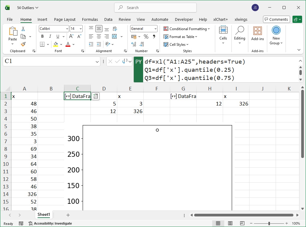
Figure 5-56 Finding Outliers

Data Transformation

To eliminate the effects of scale and magnitude, or to meet statistical method requirements, data often needs transformation before analysis. Common methods include log transform, square root transform, arcsine transform, centering, standardization, and normalization. Log and sqrt transforms can be done via column operations (Section 5.1.1). This section focuses on standardization and normalization.

Standardization: Subtract the mean from each value and divide by the standard deviation. Result: mean = 0, std = 1.

Normalization: Scale values to the range [0, 1]. Formula: (value − min) / (max − min).

In the worksheet shown in Figure 5-57, column A contains data to be standardized and normalized. In cell C1:

df = xl("A1:A85", headers=True)
ser1 = df['x']
ser2 = (ser1 - ser1.mean()) / ser1.std()

Press Ctrl+Enter. Cell C1 returns a Series (column C in Figure 5-57) — standardized data (mean 0, std 1).

For normalization (cell F1):

ser3 = (ser1 - ser1.min()) / (ser1.max() - ser1.min())

Press Ctrl+Enter. Cell F1 returns a Series (column F in Figure 5-57) — normalized data in [0, 1].

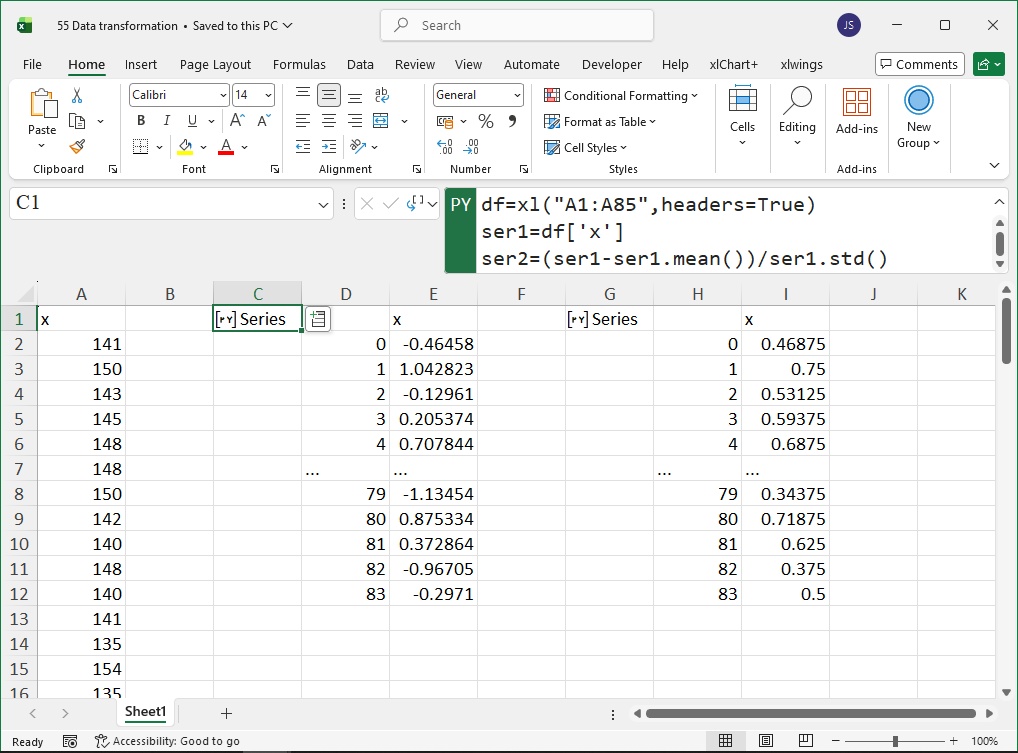
Figure 5-57 Transforming Data