Common Data Organization

Column Operations

Column operations are the most common operations for tabular data, including adding columns, transforming columns, inserting columns, creating new columns based on conditions, renaming columns, modifying column values, changing column data types, adjusting column display formats, and deleting columns.

As shown in Figure 5-1, the first three columns of the worksheet contain given data, representing the x-coordinate, y-coordinate, and radius of a series of circles. The task is to add a column for the area of the circle. There are multiple ways to calculate the area; four methods are illustrated below.

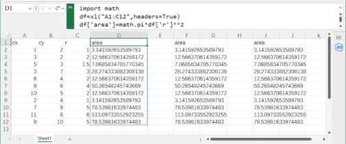
Figure 5-1

In Figure 5-1, click cell D1, enter =PY( in the formula bar to enter Python mode, and input the following code to calculate the "area" column using the mathematical formula (area = π × radius²):

import math  # Import the math package
df = xl("A1:C12", headers=True)  # Reference data
df['area'] = math.pi * df['r'] ** 2  # Calculate circle area and add new column "area"
df.area  # Reference the "area" column

Press Ctrl+Enter to get the data in column D of Figure 5-1. This method directly uses radius column data for calculation, leveraging vector operations for results.

Using apply with Lambda Function

In cell F1, enter the following code in Python mode to calculate the area using apply with a lambda function:

df['area'] = df['r'].apply(lambda x: math.pi * x ** 2)

Using transform with Lambda Function

In cell I1, enter the following code in Python mode to calculate the area using transform with a lambda function:

df['area'] = df['r'].transform(lambda x: math.pi * x ** 2)

Using Custom Functions with apply or transform

Define a custom function carea to calculate the area, then call it with apply or transform. In cell D1 (Figure 5-2), input:

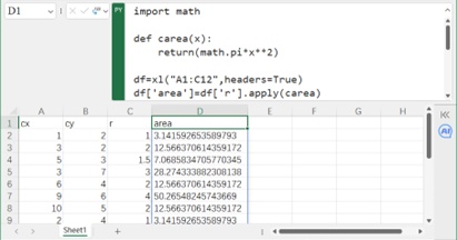
Figure 5-2

import math
def carea(x):
    return math.pi * x ** 2  # Custom function to calculate area
df = xl("A1:C12", headers=True)
df['area'] = df['r'].apply(carea)  # Use custom function "carea" to generate new column "area"
df.area

Creating New Columns Based on Conditions

In Figure 5-3, classify circles by radius:

Radius ≤ 3: Small

3 < Radius ≤ 5: Medium

Radius > 5: Large

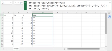
Figure 5-3

In cell D1, input the following code in Python mode:

df = xl("A1:C12", headers=True)
df['size'] = pd.cut(df['r'], [0, 3, 5, 10], labels=['Small', 'Medium', 'Large'])  # Use cut() to convert continuous data to categorical
df.loc[:, 'size']  # Reference the "size" column

This uses pd.cut() to convert sorted continuous data into categorical data.

Renaming Columns

Rename columns "cx", "cy", and "r" to "Center X Coordinate", "Center Y Coordinate", and "Radius", respectively. In cell D1 (Figure 5-4), input:

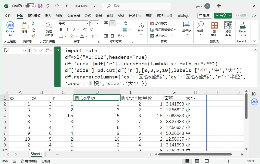
Figure 5-4

import math
df = xl("A1:C12", headers=True)
df['area'] = df['r'].transform(lambda x: math.pi * x ** 2)  # Add "area" column
df['size'] = pd.cut(df['r'], [0, 3, 5, 10], labels=['Small', 'Medium', 'Large'])  # Add "size" column
# Rename columns using a dictionary
df.rename(columns={'cx': 'Center X Coordinate', 'cy': 'Center Y Coordinate', 'r': 'Radius', 'area': 'Area', 'size': 'Size'})

Changing Column Data Types

Convert the "area" column to string type. In cell D1 (Figure 5-5), input:

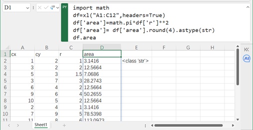
Figure 5-5

import math
df = xl("A1:C12", headers=True)
df['area'] = df['r'].transform(lambda x: math.pi * x ** 2)
df['area'] = df['area'].astype(str)  # Convert "area" to string type

Row Operations

Common row operations include adding rows directly, calculating new rows, inserting rows, modifying row names, updating row data, and deleting rows. Below is an example of calculating a new row.

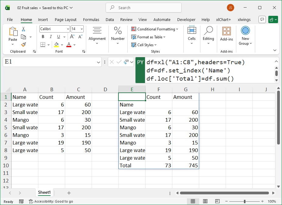
Figure 5-6

In Figure 5-6, the first three columns contain sales data for fruits. The task is to add a "Total" row at the bottom to calculate total sales volume and amount. In cell E1, input the following code in Python mode:

df = xl("A1:C8", headers=True)
df = df.set_index('Product Name')  # Set "Product Name" as the index column
df.loc['Total'] = df.sum()  # Add "Total" row using sum() to calculate column totals
df  # Output the DataFrame

Data Sorting

In Figure 5-7, sort salary data by "Net Salary" (primary) and "Gross Salary" (secondary) in ascending order. In cell K1, input:

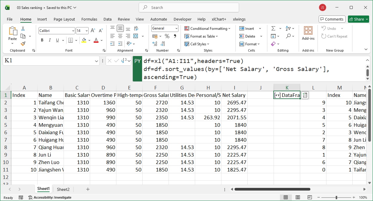
Figure 5-7

df = xl("A1:I11", headers=True)
df = df.sort_values(by=['Net Salary', 'Gross Salary'], ascending=True)  # Multi-condition sorting

Data Filtering

In Figure 5-8, filter data to include only individuals older than 25 with a bachelor’s degree. In cell E1, input:

Figure 5-8

df = xl("A1:C11", headers=True)
df[(df['Age'] > 25) & (df['Education'] == 'Bachelor')]  # Boolean indexing for filtering

Data Ranking

Rank students by exam scores using different methods (Chinese-style, American-style, etc.). In Figure 5-9, rank scores in descending order (higher scores first) using rank() with method='min' (Chinese-style ranking). In cell D1, input:

Figure 5-9

df = xl("A1:B9", headers=True)
df['Rank'] = (100 - df['Score']).rank(method='min').astype(int)  # Convert to integer to avoid decimals
df = df.sort_values(by=['Rank'], ascending=True)  # Sort by rank

American-style ranking (method='average'): Average ranks for ties.

Max ranking (method='max'): Maximum rank for ties.

First ranking (method='first'): Rank by first occurrence in raw data.

Dense ranking (method='dense'): Consecutive ranks after ties.

Random Sampling

Randomly sample 10 orders from 107 orders (Figure 5-14). In cell J1, input:

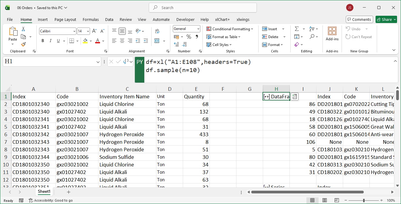
Figure 5-14

df = xl("A1:E108", headers=True)
df.sample(n=10)  # Sample 10 rows

To sample from a single column (e.g., "Order ID"):

df['Order ID'].sample(n=10)  # Sample 10 values from "Order ID" column

Wide-to-Long Table Transformation

Convert a wide table (Figure 5-15) to a long table using melt(). In cell E1, input:

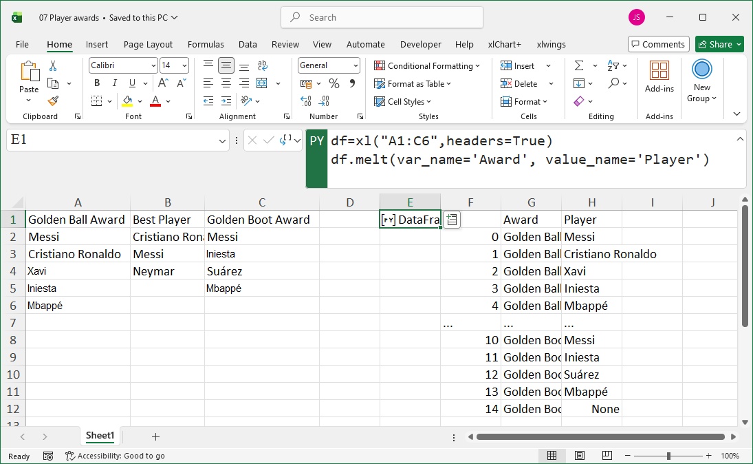
Figure 5-15

df = xl("A1:C6", headers=True)
df.melt(var_name='Award', value_name='Player')  # Reshape wide to long

Exploding Data

Explode a Series containing lists/tuples into individual elements using explode(). In cell B1 (Figure 5-16), input:

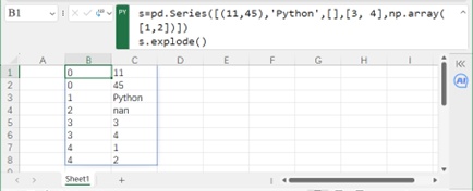
Figure 5-16

s = pd.Series([(11, 45), 'Python', [], [3, 4], np.array([1, 2])])
s.explode()  # Explode nested elements

Merging Multiple Tables

Merge data from three worksheets (Chinese, Math, English scores) using pd.merge(). In cell A1 (Figure 5-18), input:

Figure 5-18

df1 = xl("Sheet1!A1:B9", headers=True)  # Chinese scores
df2 = xl("Sheet2!A1:B9", headers=True)  # Math scores
df3 = xl("Sheet3!A1:B9", headers=True)  # English scores
merged_df = pd.merge(df1, df2, on='Name', how='outer')  # Merge first two tables
merged_df = pd.merge(merged_df, df3, on='Name', how='outer')  # Merge with third table